Beta-Amyloid Plaque Detection

Workflow Overview

This section pertains to mouse brain lightsheet data, in effort to quantify the locations and sizes of plaques in a mouse brain lightsheet scan image.

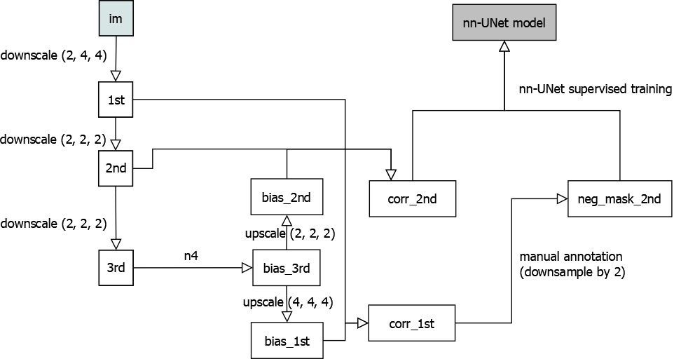
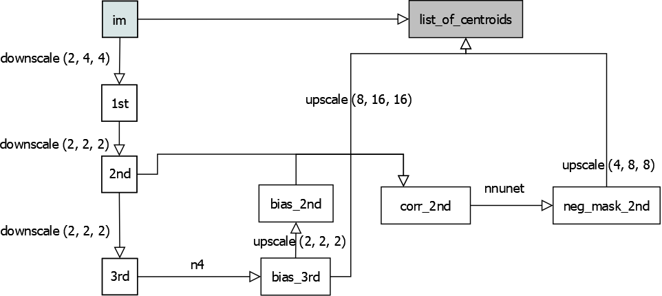
Below are figures illustrating an overview of the training and prediction stages of the pipeline, ultimately processing image volumes each to a list of centroids:

training workflow, overview

prediction workflow, overview

Things to note:

1. n4 calculation is calculated at third downsample (i.e. (8, 16, 16) times downsampled compared to original) level as the n4 bias correction is a smooth operation insensitive to small location change. It runs slowly on large images so easier to work with using a smaller input.

2. The final step of prediction workflow involves 3 inputs: Original full resolution image, third downsampled bias image, and second downsampled negative mask prediction. The image is first masked by upsampled negative mask, then corrected by the upsampled bias image. Finally, the corrected image is used to compute the list of centroids.

3. The goal of the training workflow is to obtain the model file; after which the model file may be uploaded to cloud to be downloaded somewhere else where prediction workflow needs to be run. Unlike other operations that can be done on cloud, nn-UNet predicts on local files and write to a local output location (though you can write a wrapper that wires the input and output to cloud locations).

4. Rather than nearest neighbor, downsampling is done using max-pooling to avoid a shift in image origin location after downsampling. For up-sampling, this is not an issue.

Python Implementation

For more information about nn-UNet related annotation, training and prediction, refer to the nn-UNet page.

Below draws example from the file cvpl_tools/examples/mousebrain_processing.py to explain how various steps in the above diagram is done via code. We start with an image on network in OME ZARR file and would like to obtain a final counting of list of centroids of where plaques are at.

• Downsampling

print(f'first downsample: from path {subject.OME_ZARR_PATH}')
first_downsample = lightsheet_preprocess.downsample(
    subject.OME_ZARR_PATH, reduce_fn=np.max, ndownsample_level=(1, 2, 2), ba_channel=subject.BA_CHANNEL,
    write_loc=subject.FIRST_DOWNSAMPLE_PATH
)
print(f'first downsample done. result is of shape {first_downsample.shape}')

second_downsample = lightsheet_preprocess.downsample(
    first_downsample, reduce_fn=np.max, ndownsample_level=(1,) * 3,
    write_loc=subject.SECOND_DOWNSAMPLE_PATH
)

Here, lightsheet_preprocess.downsample is a function that outputs a dask array, and also writes to local disk at write_loc. This location can be either local or on a gcs cloud bucket. Writing to cloud allow us to switch coiled cloud computing if needed, as the file location is not bound to our local laptop.

BA_CHANNEL stands for beta-amyloid channel, which is an integer selecting the channel of the image we want to process. the downsample function takes this parameter for 4d images, but can skip for 3d images.

• n4

import cvpl_tools.nnunet.n4 as n4

third_downsample_bias = await n4.obtain_bias(third_downsample, write_loc=subject.THIRD_DOWNSAMPLE_BIAS_PATH)
print('third downsample bias done.')

print(f'im.shape={second_downsample.shape}, bias.shape={third_downsample_bias.shape}; applying bias over image to obtain corrected image...')
second_downsample_bias = dask_ndinterp.scale_nearest(third_downsample_bias, scale=(2, 2, 2),
                                                     output_shape=second_downsample.shape, output_chunks=(4, 4096, 4096)).persist()

second_downsample_corr = lightsheet_preprocess.apply_bias(second_downsample, (1,) * 3, second_downsample_bias, (1,) * 3)
asyncio.run(ome_io.write_ome_zarr_image(subject.SECOND_DOWNSAMPLE_CORR_PATH, da_arr=second_downsample_corr, MAX_LAYER=1))
print('second downsample corrected image done')

coiled_run can be used instead if local laptop can not install antspyx library, as follows:

async def compute_bias(dask_worker):
    third_downsample = ome_io.load_dask_array_from_path(subject.THIRD_DOWNSAMPLE_PATH, mode='r', level=0)
    await n4.obtain_bias(third_downsample, write_loc=subject.THIRD_DOWNSAMPLE_BIAS_PATH)
if not RDirFileSystem(subject.THIRD_DOWNSAMPLE_BIAS_PATH).exists(''):
    cvpl_nnunet_api.coiled_run(fn=compute_bias, nworkers=1, local_testing=False)
third_downsample_bias = ome_io.load_dask_array_from_path(subject.THIRD_DOWNSAMPLE_BIAS_PATH, mode='r', level=0)

• upscale

second_downsample_bias = dask_ndinterp.scale_nearest(third_downsample_bias, scale=(2, 2, 2),
                                                     output_shape=second_downsample.shape, output_chunks=(4, 4096, 4096)).persist()

This step takes apparently redundant output_shape parameter alongside scale and the pre-scaled image. However, downscale and upscale often has to deal with integer division issues, while the scale is whole number, the larger image size may not be a perfect multiple of the size of the image to be scaled. output_shape adjusts for this by crop or pad the resulting image with zeros.

• uploading bias and negative mask

if not RDirFileSystem(subject.GCS_NEG_MASK_TGT).exists(''):
    cvpl_nnunet_api.upload_negmask(
        subject.NNUNET_OUTPUT_TIFF_PATH,
        subject.GCS_NEG_MASK_TGT,
        subject.THIRD_DOWNSAMPLE_BIAS_PATH,
        f'{subject.SUBJECT_FOLDER}/.temp',
        subject.GCS_BIAS_PATH
    )

This is an intermediate step not drawn in the diagram. It simply uploads the bias image and nn-UNet output negative mask to cloud, since those are computed locally in mousebrain_processing.py

• computing list of centroids

ppm_to_im_upscale = (4, 8, 8)
async def fn(dask_worker):
    await cvpl_nnunet_api.mousebrain_forward(
        dask_worker=dask_worker,
        CACHE_DIR_PATH=subject.COILED_CACHE_DIR_PATH,
        ORIG_IM_PATH=subject.OME_ZARR_PATH,
        NEG_MASK_PATH=subject.GCS_NEG_MASK_TGT,
        GCS_BIAS_PATH=subject.GCS_BIAS_PATH,
        BA_CHANNEL=subject.BA_CHANNEL,
        MAX_THRESHOLD=subject.MAX_THRESHOLD,
        ppm_to_im_upscale=ppm_to_im_upscale
    )
cvpl_nnunet_api.coiled_run(fn=fn, nworkers=10, local_testing=False)

ppm_to_im_upscale is the scale from negative mask image to the size of the original image. This is the final step of the prediction workflow, where we will obtain our list of centroids from gcs after running this. In a local test (without coiled, but still using gcs), we may set local_testing=True

Here, the MAX_THRESHOLD variable specifies the threshold above which objects will be counted as plaque. This threshold is applied over corrected ome zarr image based on the original image and bias image provided.

After running the above code, a numpy file will be written to f'{subject.COILED_CACHE_DIR_PATH}/final_lc.npy', which contains the results in a N * 5 matrix of type np.float64. First three columns are the Z, Y, X locations of the plaques, and the fourth and fifth column are sizes (in voxels) and a unique ID for the plaque. To retrieve:

from cvpl_tools.fsspec import RDirFileSystem
cdir_fs = RDirFileSystem(subject.COILED_CACHE_DIR_PATH)
with cdir_fs.open('final_lc.npy', mode='rb') as fd:
    lc = np.load(cdir_fs)
print(f'First 10 rows of lc:\n')
print(lc[:10])

Alternatively, use cvpl_tools.fsspec.copyfile function to obtain the .npy file locally.